10 Excel 2013 Advanced Formulas and Functions: Master Data Analysis With Pro-Level Techniques

Tired of cluttering your spreadsheet with helper columns just to return multiple results? Array formulas in Excel 2013 let you extract or analyze data dynamically—all within a single cell. This is your secret weapon for financial modeling, where you might need to pull top 5 sales figures or calculate moving averages without extra rows.

To use them, press Ctrl+Shift+Enter (not just Enter) to create the array. For example, {=SMALL(Table1[Sales],ROW(INDIRECT("1:5")))} pulls the top 5 sales values in one go. You can also combine functions like SUM or AVERAGE with IF inside arrays for conditional calculations. Excel 2013’s arrays work best with static ranges (no volatile functions like TODAY), but they’re perfect for extracting trends from large datasets.

Financial analysts and data crunchers will love this for consolidating reports without manual copying. Start with simple examples like ranking values before tackling multi-step array logic. ✨

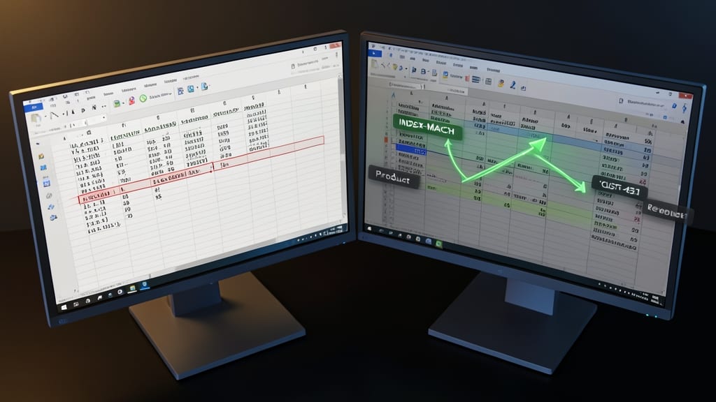
Tired of VLOOKUP’s limitations—like rigid column positions or limited horizontal lookups? The INDEX-MATCH combo is your upgrade, offering unmatched flexibility for retrieving data from any direction in your tables.

Here’s how it works: MATCH locates the position of a value (like a customer ID), while INDEX fetches the corresponding data from that spot—whether it’s in the same row, column, or even a different sheet. No more worrying about column order or duplicate headers. For example, =INDEX(B2:B100, MATCH("Smith", A2:A100, 0)) pulls "Smith’s" data from column B without fuss.

This is the go-to for analysts merging datasets or pulling specific values from large tables. If you’re juggling sales data, inventory, or multi-sheet reports, this pair will save you hours. ✨

Tired of manually adding up rows that meet specific criteria? SUMIFS and SUMIF let you filter sums by conditions—like calculating total sales for a product line in a specific region or summing inventory costs above a threshold.

With SUMIFS, you can apply up to 127 conditions (in Excel 2013) to refine your calculations, while SUMIF handles single criteria. Both functions support text, numbers, dates, and even wildcard matches, making them perfect for dynamic reports. For example, =SUMIFS(B2:B100, A2:A100, "Q3", C2:C100, ">500") sums only Q3 sales over $500.

Small business owners and analysts will love these for automating financial summaries—no more copying and pasting filtered data. ⚡

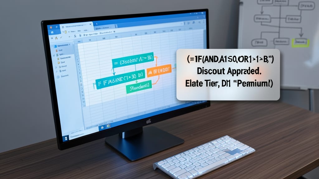
Tired of juggling multiple AND/OR conditions in your formulas? Nested IF statements let you build multi-layered logic—like a flowchart inside Excel—without writing a single line of VBA. This is your go-to for scenarios where one condition depends on another, such as tiered discounts or grading scales with multiple thresholds.

The syntax is straightforward: `=IF(logicaltest, valueiftrue, IF(logicaltest2, valueiftrue2, valueiffalse))`. For example, a grading system could check if a score is ≥90 first, then ≥80, and finally ≥70, assigning letter grades accordingly. Excel 2013 supports up to 64 nested IFs per formula, though deeper nesting can slow performance on large datasets.

Perfect for educators, sales teams, or analysts who need to automate decision-making workflows. Just remember to use IFS (Excel 2016+) for cleaner code if you upgrade—this method works flawlessly in Excel 2013 for now. ✨

Tired of manually combining or splitting text in Excel? The TEXTJOIN and CONCAT functions are your dynamic text manipulation power tools. With TEXTJOIN, you can merge cells with a custom delimiter (like commas or spaces) while ignoring empty cells—ideal for generating lists or reports. CONCAT, meanwhile, simply joins text without options, making it perfect for quick merges.

Use TEXTJOIN to clean messy datasets by combining first/last names or merging product descriptions. For example, =TEXTJOIN(", ", TRUE, A2:A10) turns a list of items into a comma-separated string. CONCAT shines when you need to append text from multiple cells, like =CONCAT(B2, " ", C2) to combine first and last names. Both functions work seamlessly in Excel 2013, saving hours of manual work.

Marketing teams will love TEXTJOIN for automating email templates, while operations staff can use it to standardize data formats. Try these today to streamline your workflows! ✨

Tired of manually adjusting dates or guessing project deadlines? EOMONTH and WORKDAY are your new time-saving power tools in Excel 2013. These functions streamline scheduling by handling calendar quirks—like month-end dates and weekends—automatically, so you never miss a deadline again.

The EOMONTH function returns the last day of a month, even if the input date is the 15th or 30th. For example, =EOMONTH("1/15/2023", 2) instantly gives you March 31, 2023, without manual counting. Meanwhile, WORKDAY adds a specified number of workdays (excluding weekends and holidays) to a start date, making it perfect for project timelines. Combine them to calculate end-of-quarter reports or holiday-adjusted deadlines in seconds.

HR managers, project leads, and finance teams will love these for automating payroll cycles, leave approvals, or budget forecasting. No more guessing—just precise, automated scheduling. ✨

Tired of Excel formulas crashing your reports with cryptic error messages like #DIV/0! or #N/A? IFERROR and ISERROR are your secret weapons for keeping calculations clean and professional.

Use IFERROR to replace error values with custom text or zeros, like =IFERROR(A1/B1, "Error"). For deeper control, ISERROR checks if a value is an error, letting you handle specific cases—perfect for financial models where precision matters. Both work in Excel 2013 and require zero add-ins.

Accountants, analysts, and dashboard builders will love these for polishing automated reports. They’re the unsung heroes of data integrity. ✨

Tired of cluttering your spreadsheets with helper columns just to filter and sort data? Excel 2013’s FILTER and SORT functions spill dynamic arrays directly into your cells, eliminating the need for extra columns and keeping your workspace clean.

With FILTER, you can extract specific rows based on conditions (e.g., =FILTER(A2:B10, A2:A10="Active")), while SORT rearranges data by column (e.g., =SORT(A2:B10, 2, -1) for descending order). The best part? These functions update automatically when your source data changes—no manual recalculations needed.

Perfect for analysts, project managers, or anyone building interactive dashboards, this combo cuts down on manual work and keeps your data analysis dynamic. ✨

If you’ve ever wondered whether an investment is truly worth the risk, NPV (Net Present Value) and IRR (Internal Rate of Return) are your secret weapons. These functions let you compare cash flows over time, factoring in the time value of money—no financial degree required.

The NPV function evaluates the present value of future cash flows using a discount rate, while IRR calculates the exact rate that makes the net present value zero. For example, =NPV(0.1, B2:B10) converts future earnings into today’s dollars, while =IRR(B2:B10) reveals the true profitability of a project. Both work seamlessly with Excel 2013’s financial toolkit, even handling irregular cash flow patterns.

Accountants, startup founders, and budget analysts will find these indispensable for evaluating loans, comparing investment opportunities, or forecasting long-term revenue. Master them, and you’ll make smarter financial decisions faster. ✨

Tired of Excel’s built-in functions not quite cutting it for your unique workflow? VBA Macros let you create custom functions that act like native Excel tools—without needing to code for every task. Whether it’s calculating niche business metrics or automating data cleanup, VBA bridges the gap between what Excel offers and what you actually need.

With VBA Editor (accessed via Developer tab), you can write functions like =MyCustomCalc(data) that run instantly in your spreadsheets. Need a tax formula for a specific region? A custom rounding rule for inventory? VBA handles it—even with error handling and input validation to keep your macros robust. Plus, record macros to auto-generate code for repetitive tasks, then tweak it for precision.

This is the go-to tool for accountants crunching specialized numbers, analysts merging disparate datasets, or small business owners automating invoices. Start with simple macros, then level up to full-blown custom functions—your workflow will thank you. 💻